
| 일 | 월 | 화 | 수 | 목 | 금 | 토 |
|---|---|---|---|---|---|---|
| 1 | 2 | 3 | 4 | 5 | ||
| 6 | 7 | 8 | 9 | 10 | 11 | 12 |
| 13 | 14 | 15 | 16 | 17 | 18 | 19 |
| 20 | 21 | 22 | 23 | 24 | 25 | 26 |
| 27 | 28 | 29 | 30 |
- subplot
- type hints
- 가능도
- Operation function
- VSCode
- Numpy
- Array operations
- python 문법
- 최대가능도 추정법
- Python 유래
- 딥러닝
- dtype
- boolean & fancy index
- 카테고리분포 MLE
- scatter
- groupby
- Numpy data I/O
- Python
- linalg
- ndarray
- 부스트캠프 AI테크
- pivot table
- Comparisons
- seaborn
- namedtuple
- unstack
- Python 특징
- BOXPLOT
- 표집분포
- 정규분포 MLE
- Today
- Total
또르르's 개발 Story
[11-3] MLP using PyTorch 본문
1️⃣ 설정
1) device 설정 : GPU 사용 or CPU 사용
device = torch.device('cuda:0' if torch.cuda.is_available() else 'cpu')
2) Dataset 가지고 오기
PyTorch에서는 기본적으로 datasets를 지원합니다.
from torchvision import datasets,transformstrain시킬 데이터를 tensor형태로 불러옵니다.
mnist_train = datasets.MNIST(root='./data/',train=True,transform=transforms.ToTensor(),download=True)test할 데이터를 tensor형태로 불러옵니다.
mnist_test = datasets.MNIST(root='./data/',train=False,transform=transforms.ToTensor(),download=True)
3) DataLoader : 데이터를 가지고와 generator 형태로 저장
DataLoader을 사용해서 mnist_train data를 BATCH_SIZE만큼 섞어서 불러옵니다.
train_iter = torch.utils.data.DataLoader(mnist_train,batch_size=BATCH_SIZE,shuffle=True,num_workers=1) #num_workers는 멀티프로세스 몇개 사용할 것인지DataLoader을 사용해서 mnist_test data를 BATCH_SIZE만큼 섞어서 불러옵니다.
test_iter = torch.utils.data.DataLoader(mnist_test,batch_size=BATCH_SIZE,shuffle=True,num_workers=1)
2️⃣ MLP 모델
1) MLP Model
class MultiLayerPerceptronClass(nn.Module):

    def __init__(self,name='mlp',xdim=784,hdim=256,ydim=10):	# x dimension, hidden dimension, y dimension

        super(MultiLayerPerceptronClass,self).__init__()	# MultiLayerPerceptronClass의 init 상속

        self.name = name

        self.xdim = xdim

        self.hdim = hdim

        self.ydim = ydim

        self.lin_1 = nn.Linear(self.xdim, self.hdim)		# 1 layer로 xdim 입력 -> hdim 출력

        self.lin_2 = nn.Linear(self.hdim, self.ydim)		# 2 layer로 hdim 입력 -> ydim 출력

        self.init_param() # initialize parameters


    def init_param(self):

        nn.init.kaiming_normal_(self.lin_1.weight)		# 정규분포를 이용해서 weight 초기화

        nn.init.zeros_(self.lin_1.bias)				# bias 0으로 초기화

        nn.init.kaiming_normal_(self.lin_2.weight)

        nn.init.zeros_(self.lin_2.bias)


    def forward(self,x):

        net = x

        net = self.lin_1(net)					# 1번 수행

        net = F.relu(net)					# 활성함수

        net = self.lin_2(net)					# 2번 수행

        return net
2) loss & optimizer
Class를 선언하고 device (cuda)에 올려줍니다.
이때, x 입력 차원을 784, hidden layer 차원을 256, y 출력 차원을 10을 선업합니다.
M = MultiLayerPerceptronClass(name='mlp',xdim=784,hdim=256,ydim=10).to(device)Loss는 CrossEntroyLoss를 사용합니다. (PyTorch에서 제공)
loss = nn.CrossEntropyLoss()Optimizer는 Adam을 사용합니다. learn rate를 설정해주어야합니다.
optm = optim.Adam(M.parameters(),lr=1e-3)
3) Model Parameter 확인
np.set_printoptions(precision=3)    # numpy float 출력옵션 변경

n_param = 0

for p_idx,(param_name,param) in enumerate(M.named_parameters()):

    param_numpy = param.detach().cpu().numpy()    # detach() : 기존 Tensor에서 gradient 전파가 안되는 텐서 생성

    n_param += len(param_numpy.reshape(-1))		# 한줄로 만들어줌

    print ("[%d] name:[%s] shape:[%s]."%(p_idx,param_name,param_numpy.shape))

    print ("    val:%s"%(param_numpy.reshape(-1)[:5]))

print ("Total number of parameters:[%s]."%(format(n_param,',d')))		# 총 parameter 수


[0] name:[lin_1.weight] shape:[(256, 784)].
    val:[-0.008 -0.008 -0.01  -0.019  0.035]
[1] name:[lin_1.bias] shape:[(256,)].
    val:[0. 0. 0. 0. 0.]
[2] name:[lin_2.weight] shape:[(10, 256)].
    val:[ 0.023  0.031 -0.043 -0.035 -0.074]
[3] name:[lin_2.bias] shape:[(10,)].
    val:[0. 0. 0. 0. 0.]
Total number of parameters:[203,530].
detach() : 기존 Tensor에서 gradient 전파가 안되는 텐서 생성
(단, storage를 공유하기에 detach로 생성한 Tensor가 변경되면 원본 Tensor도 똑같이 변함)
param_numpy = param.detach().cpu().numpy() # detach() : 기존 Tensor에서 gradient 전파가 안되는 텐서 생성
3️⃣ Evaluation Function
1) Evaluation Function
def func_eval(model,data_iter,device):

    with torch.no_grad():     # gradients를 업데이트X

        model.eval() # evaluate (affects DropOut and BN)

        n_total,n_correct = 0,0

        for batch_in,batch_out in data_iter:    # batch_in=data, batch_out=label

            y_trgt = batch_out.to(device)

            model_pred = model(batch_in.view(-1, 28*28).to(device))

            _,y_pred = torch.max(model_pred.data,1)

            n_correct += (

                (y_pred==y_trgt)  # y와 y hat 값을 비교 후, sum

            ).sum().item()

            n_total += batch_in.size(0)

        val_accr = (n_correct/n_total)

        model.train() # back to train mode

    return val_accr

print ("Done")
torch.no_grad()는 Gradients를 업데이트 하지 않습니다.
with torch.no_grad(): # gradients를 업데이트XEvaluation Function에서는 model.eval()과 model.train() 모드를 바꿔주는 것이 중요합니다.
model.eval() # evaluate (affects DropOut and BN)

...

model.train() # back to train mode
DataLoader에서 가지고 온 data_iter이며, train_iter와 test_iter가 존재합니다.
MNIST에서 batch_in은 data (28 x 28 x 256의 tensor)와 batch_out은 label (1 x 256 tensor)로 되어있습니다.
for batch_in,batch_out in data_iter: # batch_in=data, batch_out=labelbatch_out은 정답 label이기 때문에 y_trgt 변수에 저장합니다.
y_trgt = batch_out.to(device)Linear에서 X input이 28*28 = 784로 고정되어있기 때문에 일자로 펴서 넣어줍니다.
model_pred = model(batch_in.view(-1, 28*28).to(device))torch.max 함수는 주어진 텐서 배열의 최대 값이 들어있는 index를 리턴하는 함수입니다.
torch.max(model_pred.data,1)에서 1은 1번째 dimension 기준으로 max 값을 출력하라는 의미입니다.
만약 1을 사용하지 않는다면 기준 없이 전체 값 중 max를 찾게 됩니다.
>>> print(torch.max(model_pred.data))

tensor(1.8898, device='cuda:0')
하지만 1을 추가한다면 axis=1 방향으로 max값을 계산하게 됩니다.
>>> print(torch.max(model_pred.data,1))

torch.return_types.max(
values=tensor([0.4602, 0.3046, 0.6478, 0.3857, 0.5591, 0.3893, 0.4803, 0.2910, 0.3256,
        0.4420, 0.3038, 0.3905, 0.4485, 0.5423, 0.1953, 0.2711, 1.5264, 0.6142,
        0.5271, 0.4416, 0.4385, 0.9487, 0.5373, 0.2716, 0.3867, 0.2307, 1.2070,
        0.4033, 0.4818, 0.4699, 0.5011, 0.3498, 0.2141, 0.5532, 0.2601, 0.3380,
        0.8151, 0.2346, 0.3442, 0.2818, 0.4904, 0.2673, 0.5763, 0.4272, 0.5062,
        0.3532, 0.2523, 0.6189, 0.3370, 0.5919, 0.6986, 0.2846, 0.3234, 0.6096,
        0.2306, 0.4915, 0.3975, 0.4238, 0.2827, 0.4835, 0.6407, 0.4626, 0.9545,
        0.2115, 0.5217, 0.2483, 0.2787, 0.1835, 0.3419, 0.2275, 0.7623, 0.6255,
        0.2528, 0.2800, 0.7635, 0.5788, 0.6383, 0.1356, 0.1530, 0.3945, 0.3482,
        0.3169, 0.4676, 0.2786, 0.6458, 0.5519, 1.6937, 0.6849, 0.6407, 0.4835,
        0.5494, 0.3606, 0.2647, 0.7565, 0.2380, 0.5460, 0.6458, 0.3949, 0.1656,
        0.0837, 0.2032, 0.5707, 1.0058, 0.3713, 0.3374, 0.1981, 0.6068, 0.4134,
        0.4221, 0.3364, 0.5048, 0.5798, 0.2657, 0.4241, 0.8593, 0.3963, 0.6320,
        0.5924, 0.7194, 0.3375, 0.2539, 0.0837, 0.5846, 0.4009, 0.7050, 0.4057,
        0.3265, 0.1858, 0.2381, 0.5453, 0.3506, 0.5003, 0.4977, 1.0419, 0.4407,
        0.3030, 0.1756, 0.4114, 0.6345, 0.4114, 0.3167, 0.5588, 0.5339, 0.3262,
        0.3485, 0.2627, 0.4920, 0.2804, 0.9049, 0.6536, 0.5207, 0.7514, 0.4539,
        0.3613, 0.2599, 0.3705, 0.2586, 0.6514, 1.3507, 0.6036, 0.9566, 0.2534,
        0.7953, 0.5072, 0.6334, 1.1344, 0.4369, 0.3927, 0.1374, 0.6042, 0.5445,
        0.4933, 1.2110, 0.4883, 0.0361, 0.2184, 0.9502, 0.5470, 0.4957, 0.5596,
        0.5820, 1.4527, 0.7928, 0.1329, 0.4296, 0.3009, 0.3631, 0.3168, 1.1965,
        0.3300, 0.2656, 0.6038, 0.8363, 0.6407, 0.3385, 0.2552, 0.3876, 0.7898,
        0.2833, 0.1174, 0.2028, 0.4573, 0.3614, 0.3428, 0.4718, 0.2701, 0.3558,
        0.4324, 0.3354, 0.5030, 0.4348, 0.5266, 0.8746, 0.5431, 0.3429, 0.1024,
        0.4958, 0.3307, 0.4702, 0.1502, 0.5989, 0.3853, 0.6414, 0.4651, 0.7332,
        0.2669, 0.4120, 0.7751, 0.7475, 0.2735, 0.2571, 0.3781, 0.4809, 0.7821,
        0.5192, 0.5137, 0.4892, 0.5874, 0.6481, 0.4441, 0.1637, 0.1393, 0.4743,
        0.2966, 0.2008, 0.6737, 0.1558, 0.5252, 0.3077, 0.1716, 0.4760, 0.4320,
        0.3435, 0.2351, 0.8363, 0.3863], device='cuda:0'),
indices=tensor([6, 4, 1, 5, 8, 4, 8, 6, 8, 5, 8, 1, 4, 9, 5, 5, 6, 6, 0, 6, 5, 4, 4, 6,
        5, 4, 6, 5, 6, 8, 6, 4, 4, 6, 6, 9, 1, 8, 6, 5, 8, 5, 4, 9, 6, 8, 5, 8,
        8, 4, 1, 9, 6, 6, 5, 6, 5, 4, 8, 8, 9, 8, 6, 6, 6, 8, 6, 4, 8, 1, 6, 5,
        5, 0, 1, 9, 6, 9, 8, 4, 6, 4, 6, 1, 6, 5, 6, 4, 4, 4, 4, 0, 6, 4, 4, 4,
        6, 4, 4, 0, 8, 0, 6, 4, 6, 0, 6, 4, 8, 1, 5, 5, 4, 5, 6, 8, 4, 5, 5, 9,
        1, 4, 6, 4, 4, 5, 5, 8, 5, 4, 4, 5, 6, 6, 4, 0, 8, 5, 6, 6, 0, 4, 6, 5,
        8, 8, 5, 8, 6, 4, 5, 6, 4, 0, 0, 6, 4, 6, 6, 5, 6, 5, 6, 4, 6, 6, 4, 9,
        8, 6, 6, 4, 6, 4, 8, 6, 6, 4, 9, 5, 9, 6, 6, 1, 0, 9, 6, 4, 6, 4, 6, 6,
        6, 6, 6, 4, 5, 4, 5, 0, 6, 6, 6, 0, 4, 4, 6, 8, 4, 6, 9, 6, 6, 4, 4, 4,
        6, 8, 1, 5, 6, 6, 5, 9, 6, 4, 5, 4, 5, 8, 6, 5, 1, 0, 1, 0, 8, 6, 1, 6,
        5, 4, 4, 2, 0, 1, 1, 4, 5, 0, 1, 9, 4, 8, 4, 6], device='cuda:0'))
따라서 torch.max의 첫번째 return은 max값, 두 번째 return은 max index값을 나타냅니다.
>>> val,y_pred = torch.max(model_pred.data,1)

>>> print(val)

>>> print(y_pred)

tensor([ 0.3048,  0.1675,  0.6583,  0.4321,  0.6558,  0.4975,  0.2758,  0.7619,
         0.7811,  0.5031,  0.7324,  0.3163,  0.4983,  0.5016,  0.2352,  0.3409,
         0.3627,  0.7645,  0.3566,  0.1741,  0.3232,  1.5084,  0.4818,  0.0969,
         0.7491,  0.2785,  0.6561,  0.3747,  0.4575,  0.6766,  0.5851,  0.6253,
         0.3412,  0.2749,  0.2250,  0.1841,  0.3867,  0.3337,  0.9198,  0.5689,
         0.2622,  0.6611,  0.4949,  0.3818,  0.2049,  0.3298,  0.4685,  0.6889,
         0.6565,  0.8036,  0.3914,  0.5469,  0.5895,  0.5536,  0.3779,  0.7365,
         0.1668,  0.1770,  0.9142,  0.2929,  0.3293,  0.7898,  0.4054,  0.1251,
         0.6209,  0.2214,  0.3955,  0.5612,  0.3228,  0.3876,  0.5439,  0.0936,
         0.5762,  0.9588,  1.1368,  0.3911,  0.5195,  0.6343,  0.2449,  0.2390,
         0.1755,  0.4156,  0.7306,  0.1930,  0.4865,  0.4822,  0.9243,  0.4268,
         0.3853,  0.3839,  0.6583,  1.2110,  0.3320,  0.3775,  0.3847,  0.1298,
         0.6038,  0.6395,  0.7173,  0.2751,  0.3014,  0.4343,  0.3127,  0.6717,
         0.4465,  0.8973,  0.8898, -0.0151,  0.4935,  0.4292,  0.8346,  0.3995,
         0.2975,  0.3473,  0.6437,  0.3662,  0.3892,  0.8401,  0.5590,  0.3603,
         0.7300,  0.4528,  0.6000,  0.2193,  0.4697,  0.3789,  0.4867,  0.7637,
         0.8075,  0.2068,  0.3720,  0.2384,  0.5597,  0.3766,  0.4879,  0.6223,
         1.5516,  0.2585,  0.1832,  0.5769,  0.8798,  0.4482,  0.4191,  0.4618,
         0.3706,  0.6326,  0.5646,  0.4024,  0.7878,  1.4860,  0.3906,  0.2468,
         0.2555,  0.5379,  0.4059,  0.7265,  0.6907,  0.3905,  0.4053,  0.2808,
         0.4130,  0.7621,  0.3909,  0.3326,  0.9923,  0.1321,  0.3472,  0.7002,
         0.5815,  0.7539,  0.5688,  0.2450,  0.4044,  0.6826,  0.5593,  1.0467,
         0.8662,  0.2161,  0.0866,  0.2473,  0.5387,  0.1422,  0.3621,  0.5153,
         0.4292,  0.2601,  0.5510,  0.5207,  0.9192,  0.0831,  0.5403,  0.4091,
         0.4005,  0.2832,  0.7564,  0.3660,  0.7204,  0.4361,  0.3534,  1.0457,
         0.3160,  0.3122,  0.5551,  0.5737,  0.5776,  0.6892,  0.6044,  0.5588,
         0.5201,  0.3324,  0.5407,  0.3808,  0.4640,  0.5814,  0.4325,  0.3220,
         0.2545,  0.1475,  0.4384,  0.3319,  0.5455,  0.2629,  0.2493,  0.4548,
         0.3063,  0.6044,  0.4726,  0.3051,  0.6189,  0.7063,  0.4495,  0.3294,
         0.2978,  0.9994,  0.3499,  0.1906,  0.3270,  0.4412,  0.3816,  0.8032,
         0.7694,  0.4320,  0.5782,  0.9506,  0.3254,  0.5243,  0.4332,  0.4616,
         0.1782,  0.1623,  0.7486,  0.4836,  0.5362,  0.3929,  0.5669,  0.1780],
       device='cuda:0')
tensor([8, 9, 4, 5, 9, 5, 5, 6, 4, 8, 6, 4, 9, 0, 9, 5, 5, 6, 9, 5, 8, 6, 4, 4,
        4, 4, 5, 6, 0, 0, 5, 6, 4, 5, 8, 6, 8, 5, 6, 6, 5, 6, 8, 1, 8, 5, 8, 6,
        1, 5, 9, 5, 6, 4, 6, 4, 5, 0, 6, 8, 1, 8, 4, 8, 6, 6, 8, 6, 6, 8, 5, 5,
        6, 6, 6, 5, 4, 4, 8, 5, 5, 4, 5, 5, 6, 9, 4, 4, 5, 4, 4, 6, 8, 8, 8, 0,
        6, 6, 5, 6, 0, 5, 8, 5, 6, 0, 4, 9, 6, 6, 9, 6, 1, 9, 6, 5, 9, 6, 0, 9,
        4, 9, 4, 8, 6, 5, 4, 6, 6, 0, 5, 6, 1, 9, 5, 4, 6, 0, 8, 6, 4, 0, 4, 4,
        4, 6, 1, 2, 6, 6, 8, 9, 0, 9, 5, 0, 6, 6, 4, 6, 6, 8, 9, 0, 6, 8, 8, 6,
        4, 6, 4, 5, 8, 4, 8, 6, 6, 6, 5, 6, 5, 4, 5, 6, 1, 6, 6, 5, 6, 8, 4, 8,
        5, 5, 4, 6, 6, 6, 5, 6, 8, 9, 6, 1, 8, 5, 6, 1, 4, 8, 6, 9, 4, 0, 5, 6,
        5, 4, 1, 6, 1, 9, 9, 5, 8, 8, 6, 4, 1, 4, 6, 5, 4, 6, 9, 9, 9, 6, 5, 6,
        8, 4, 8, 6, 7, 4, 0, 5, 9, 5, 6, 5, 4, 8, 8, 1], device='cuda:0')
n_correct는 y_pred와 y_trgt 값이 같을 때만 sum을 해서 더해줍니다.
item()을 사용하면 숫자 값을 얻을 수 있습니다.
n_correct += (

	y_pred==y_trgt  # y와 y hat 값을 비교 후, sum

            ).sum().item()
n_total에다가 batch_in의 첫 번째 dimension 256을 더해줍니다.
n_total += batch_in.size(0)val_accr는 전체 데이터에서 몇 개가 맞았는지를 나타냅니다.
val_accr = (n_correct/n_total)
2) Initial Evaluation
초반 init을 해주는 과정이며, 초반에는 train_accr와 test_accr의 비율이 떨어지는 것을 알 수 있습니다.
M.init_param() # initialize parameters

train_accr = func_eval(M,train_iter,device)

test_accr = func_eval(M,test_iter,device)

>>> print ("train_accr:[%.3f] test_accr:[%.3f]."%(train_accr,test_accr))


train_accr:[0.101] test_accr:[0.099].
4️⃣ Train
print ("Start training.")

M.init_param() # initialize parameters

M.train()

EPOCHS,print_every = 10,1

for epoch in range(EPOCHS):

    loss_val_sum = 0

    for batch_in,batch_out in train_iter:

        # Forward path

        y_pred = M.forward(batch_in.view(-1, 28*28).to(device)) # 일렬로 넣어줌

        loss_out = loss(y_pred,batch_out.to(device))

        # Update

        optm.zero_grad()      # reset gradient

        loss_out.backward()      # backpropagate

        optm.step()      # optimizer update

        loss_val_sum += loss_out

    loss_val_avg = loss_val_sum/len(train_iter)

    # Print

    if ((epoch%print_every)==0) or (epoch==(EPOCHS-1)):

        train_accr = func_eval(M,train_iter,device)

        test_accr = func_eval(M,test_iter,device)

        print ("epoch:[%d] loss:[%.3f] train_accr:[%.3f] test_accr:[%.3f]."%

               (epoch,loss_val_avg,train_accr,test_accr))

print ("Done")
Start training.
epoch:[0] loss:[0.372] train_accr:[0.946] test_accr:[0.945].
epoch:[1] loss:[0.164] train_accr:[0.965] test_accr:[0.959].
epoch:[2] loss:[0.115] train_accr:[0.975] test_accr:[0.969].
epoch:[3] loss:[0.088] train_accr:[0.981] test_accr:[0.974].
epoch:[4] loss:[0.070] train_accr:[0.984] test_accr:[0.975].
epoch:[5] loss:[0.056] train_accr:[0.989] test_accr:[0.979].
epoch:[6] loss:[0.046] train_accr:[0.990] test_accr:[0.978].
epoch:[7] loss:[0.039] train_accr:[0.992] test_accr:[0.977].
epoch:[8] loss:[0.032] train_accr:[0.995] test_accr:[0.979].
epoch:[9] loss:[0.028] train_accr:[0.995] test_accr:[0.979].
Done
loss는 y_predict값과 실제 y label값의 차이를 구합니다.
loss_out = loss(y_pred,batch_out.to(device))optimizer를 사용해서 gradient를 update합니다.
이때, backward()는 loss만 계산해주고 가중치 업데이트는 하지않기 때문에, optm.step()을 통해 업데이트해주어야 합니다. optm.zero_grad()는 gradient를 reset하기 위해 사용되며, 한 번의 mini batch의 backpropagation이 끝나면, 업데이트를 해주고 reset해서 다시 사용(시작점을 동일하게 하기 위해서)합니다.
# Update

optm.zero_grad()		# reset gradient

loss_out.backward()		# backpropagate

optm.step()			# optimizer update
5️⃣ Test
n_sample = 25

sample_indices = np.random.choice(len(mnist_test.targets), n_sample, replace=False)

test_x = mnist_test.data[sample_indices]

test_y = mnist_test.targets[sample_indices]

with torch.no_grad():

    y_pred = M.forward(test_x.view(-1, 28*28).type(torch.float).to(device)/255.)

y_pred = y_pred.argmax(axis=1)

plt.figure(figsize=(10,10))

for idx in range(n_sample):

    plt.subplot(5, 5, idx+1)

    plt.imshow(test_x[idx], cmap='gray')

    plt.axis('off')

    plt.title("Pred:%d, Label:%d"%(y_pred[idx],test_y[idx]))

plt.show()

print ("Done")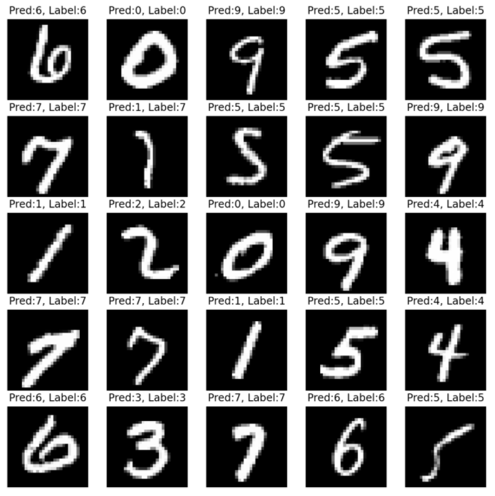
Sample의 idx를 고르는 작업입니다.
sample_indices = np.random.choice(len(mnist_test.targets), n_sample, replace=False)Model에 forward 후 나온 predict값의 argmax(index를 구함)를 출력합니다.
with torch.no_grad():

    y_pred = M.forward(test_x.view(-1, 28*28).type(torch.float).to(device)/255.)

y_pred = y_pred.argmax(axis=1)
Plt를 사용하여 image를 show합니다.
plt.figure(figsize=(10,10))

for idx in range(n_sample):

    plt.subplot(5, 5, idx+1)

    plt.imshow(test_x[idx], cmap='gray')

    plt.axis('off')

    plt.title("Pred:%d, Label:%d"%(y_pred[idx],test_y[idx]))

plt.show()
'부스트캠프 AI 테크 U stage > 실습' 카테고리의 다른 글
| [13-3] Google Image Data 다운로드 (0) | 2021.02.04 |
|---|---|
| [13-2] Colab에서 DataSet 다루기 (강아지 DataSet) (0) | 2021.02.04 |
| [13-1] CNN using PyTorch (0) | 2021.02.04 |
| [12-2] Optimizers using PyTorch (0) | 2021.02.03 |
| [02-1] Git 사용법 (0) | 2021.01.20 |


