
| 일 | 월 | 화 | 수 | 목 | 금 | 토 |
|---|---|---|---|---|---|---|
| 1 | 2 | 3 | 4 | 5 | ||
| 6 | 7 | 8 | 9 | 10 | 11 | 12 |
| 13 | 14 | 15 | 16 | 17 | 18 | 19 |
| 20 | 21 | 22 | 23 | 24 | 25 | 26 |
| 27 | 28 | 29 | 30 |
- type hints
- ndarray
- 표집분포
- Comparisons
- Numpy
- Python 유래
- Python 특징
- 정규분포 MLE
- unstack
- BOXPLOT
- 딥러닝
- VSCode
- Numpy data I/O
- 부스트캠프 AI테크
- scatter
- 가능도
- 최대가능도 추정법
- groupby
- pivot table
- 카테고리분포 MLE
- Python
- linalg
- boolean & fancy index
- namedtuple
- python 문법
- Operation function
- seaborn
- dtype
- subplot
- Array operations
- Today
- Total
또르르's 개발 Story
[14-2] LSTM using PyTorch 본문
1️⃣ 설정
1) device 설정 : GPU 사용 or CPU 사용
device = torch.device('cuda:0' if torch.cuda.is_available() else 'cpu')
2) Dataset 가지고 오기
PyTorch에서는 기본적으로 datasets를 지원합니다.
from torchvision import datasets,transformstrain시킬 데이터를 tensor형태로 불러옵니다.
mnist_train = datasets.MNIST(root='./data/',train=True,transform=transforms.ToTensor(),download=True)test할 데이터를 tensor형태로 불러옵니다.
mnist_test = datasets.MNIST(root='./data/',train=False,transform=transforms.ToTensor(),download=True)
3) DataLoader : 데이터를 가지고와 generator 형태로 저장
DataLoader을 사용해서 mnist_train data를 BATCH_SIZE만큼 섞어서 불러옵니다.
train_iter = torch.utils.data.DataLoader(mnist_train,batch_size=BATCH_SIZE,shuffle=True,num_workers=1) #num_workers는 멀티프로세스 몇개 사용할 것인지DataLoader을 사용해서 mnist_test data를 BATCH_SIZE만큼 섞어서 불러옵니다.
test_iter = torch.utils.data.DataLoader(mnist_test,batch_size=BATCH_SIZE,shuffle=True,num_workers=1)
2️⃣ LSTM 모델
1) LSTM Model
class RecurrentNeuralNetworkClass(nn.Module):

    def __init__(self,name='rnn',xdim=28,hdim=256,ydim=10,n_layer=3):

        #xdim = rnn에 입력으로 들어가는 하나의 vector

        #hdim = rnn의 hidden dims

        super(RecurrentNeuralNetworkClass,self).__init__()

        self.name = name

        self.xdim = xdim

        self.hdim = hdim

        self.ydim = ydim

        self.n_layer = n_layer # K


        self.rnn = nn.LSTM(

            #num_layers = rnn을 몇단 stack할지

            input_size=self.xdim,hidden_size=self.hdim,num_layers=self.n_layer,batch_first=True)

        # 그리고 나오는 output(self.rnn)에 linear을 추가

        self.lin = nn.Linear(self.hdim,self.ydim)


    def forward(self,x):

        # Set initial hidden and cell states (LSTM은 cell state, hidden state가 있기 때문)

        # self.n_layer는 layer을 4개 쌓았다고 하면, 4개의 LSTM에 모두 0을 넣어주어야함

        # x.size(0)은 xdim size와 똑같아야함(입력과 똑같은 dimension)

        # x는 원핫백터 h,e,l,l,0에서 [h,e,l,o]로 표현되며 [1,0,0,0], [0,1,0,0]...처럼 4x4가 됨

        # size of x : (batch_size, time_steps, input_vector_size)

        # hidden state : (num_layers, batch_size, hdim)

        h0 = torch.zeros(self.n_layer,x.size(0),self.hdim).to(device)

        c0 = torch.zeros(self.n_layer,x.size(0),self.hdim).to(device)


        # RNN

        rnn_out,(hn,cn) = self.rnn(x, (h0,c0))

        # x:[N x L x Q] => rnn_out:[N x L x D]


        # Linear

        # rnn_out[:,-1,:]에서 앞 :은 tensor에서 해당 dimension을 가지고옴

        # 앞 : 은 sequence의 마지막을 사용할 것이기 때문에 n을 그대로 사용, n개의 batch가 들어오면 n개를 병렬로

        # 중간 : 은 sequence의 마지막, 마지막 :은 D를 나타냄

        # LSTM이 돌고 나오는 결과 값

        out = self.lin(rnn_out[:,-1,:]).view([-1,self.ydim]) # [N x K] 마지막 레이어를 의미

        return out
2) loss & optimizer
Class를 선언하고 device (cuda)에 올려줍니다.
이때, x 입력 차원을 28, hidden layer 차원을 256, y 출력 차원을 10, n_layer를 2개로 선업합니다.
R = RecurrentNeuralNetworkClass(name='rnn',xdim=28,hdim=256,ydim=10,n_layer=2).to(device)Loss는 CrossEntroyLoss를 사용합니다. (PyTorch에서 제공)
loss = nn.CrossEntropyLoss()Optimizer는 Adam을 사용합니다. learn rate를 설정해주어야합니다.
optm = optim.Adam(M.parameters(),lr=1e-3)
3) Parameters Dimension 확인
Check How LSTM Works
- N: number of batches (batch 크기)
- L: sequence lengh (sequence 길이)
- Q: input dim (input 차원)
- K: number of layers (layer 수)
- D: LSTM feature dimension (LSTM feature 차원)
Y,(hn,cn) = LSTM(X)
- X: [N x L x Q] - N input sequnce of length L with Q dim.
- Y: [N x L x D] - N output sequnce of length L with D feature dim.
- hn: [K x N x D] - K (per each layer) of N final hidden state with D feature dim.
- cn: [K x N x D] - K (per each layer) of N final hidden state with D cell dim.
np.set_printoptions(precision=3)

torch.set_printoptions(precision=3)

x_numpy = np.random.rand(2,20,28) # [N x L x Q]

x_torch = torch.from_numpy(x_numpy).float().to(device)

rnn_out,(hn,cn) = R.rnn(x_torch) # forward path


print ("x_torch:", x_torch.shape) # [N x L x Q]

print ("rnn_out:",rnn_out.shape) # [N x L x D]

print ("Hidden State hn:",hn.shape) # [K x N x D]

print ("Cell States cn:",cn.shape) # [K x N x D]
x_torch: torch.Size([2, 20, 28])
rnn_out: torch.Size([2, 20, 256])
Hidden State hn: torch.Size([2, 2, 256])
Cell States cn: torch.Size([2, 2, 256])
4) Model Parameter 확인
# RNN은 parameter가 꽤 많이 들어감

# LSTM의 input gate, output gate들은 다 dense layer

# parameter을 줄일려면 hidden dimension을 줄여야함

np.set_printoptions(precision=3)

n_param = 0

for p_idx,(param_name,param) in enumerate(R.named_parameters()):

    if param.requires_grad:

        param_numpy = param.detach().cpu().numpy() # to numpy array

        n_param += len(param_numpy.reshape(-1))

        print ("[%d] name:[%s] shape:[%s]."%(p_idx,param_name,param_numpy.shape))

        print ("    val:%s"%(param_numpy.reshape(-1)[:5]))

print ("Total number of parameters:[%s]."%(format(n_param,',d')))


[0] name:[rnn.weight_ih_l0] shape:[(1024, 28)].
    val:[-0.02   0.    -0.025  0.004 -0.004]
[1] name:[rnn.weight_hh_l0] shape:[(1024, 256)].
    val:[-0.003 -0.062 -0.059 -0.056 -0.024]
[2] name:[rnn.bias_ih_l0] shape:[(1024,)].
    val:[-0.056  0.019 -0.051 -0.032 -0.035]
[3] name:[rnn.bias_hh_l0] shape:[(1024,)].
    val:[ 0.048  0.046 -0.02  -0.054  0.011]
[4] name:[rnn.weight_ih_l1] shape:[(1024, 256)].
    val:[ 0.043  0.038 -0.061 -0.054  0.019]
[5] name:[rnn.weight_hh_l1] shape:[(1024, 256)].
    val:[-0.027  0.056  0.031 -0.024  0.036]
[6] name:[rnn.bias_ih_l1] shape:[(1024,)].
    val:[ 0.012  0.016 -0.031  0.019  0.01 ]
[7] name:[rnn.bias_hh_l1] shape:[(1024,)].
    val:[ 0.     0.046 -0.039 -0.029 -0.054]
[8] name:[lin.weight] shape:[(10, 256)].
    val:[ 0.018  0.016  0.036 -0.027  0.028]
[9] name:[lin.bias] shape:[(10,)].
    val:[ 0.059 -0.034  0.055  0.039  0.025]
Total number of parameters:[821,770].
3️⃣ Evaluation Function
1) Evaluation Function
def func_eval(model,data_iter,device):

    with torch.no_grad():     # gradients를 업데이트X

        model.eval() # evaluate (affects DropOut and BN)

        n_total,n_correct = 0,0

        for batch_in,batch_out in data_iter:    # batch_in=data, batch_out=label

            y_trgt = batch_out.to(device)

            model_pred = model(batch_in.view(-1, 28, 28).to(device))

            _,y_pred = torch.max(model_pred.data,1)

            n_correct += (

                (y_pred==y_trgt)  # y와 y hat 값을 비교 후, sum

            ).sum().item()

            n_total += batch_in.size(0)

        val_accr = (n_correct/n_total)

        model.train() # back to train mode

    return val_accr

print ("Done")
2) Initial Evaluation
초반 init을 해주는 과정이며, 초반에는 train_accr와 test_accr의 비율이 떨어지는 것을 알 수 있습니다.
M.init_param() # initialize parameters

train_accr = func_eval(R,train_iter,device)

test_accr = func_eval(R,test_iter,device)

>>> print ("train_accr:[%.3f] test_accr:[%.3f]."%(train_accr,test_accr))


train_accr:[0.101] test_accr:[0.099].
4️⃣ Train
LSTM은 MNIST를 분류하는데 한 번에 한개의 row를 본 후 sequence하게 28개의 row를 본 후 예측을 수행합니다. 따라서 epoch [1]에서부터 0.94 정도의 예측률이 나오게 됩니다.
# MNIST 분류를 하는데 한번에 row 한개씩 봐서 sequence하게 28row를 보고 난 다음에 예측을 하는 것

# 그래서 epoch [1]에서도 0.94정도의 예측률이 나옴

print ("Start training.")

R.train() # to train mode

EPOCHS,print_every = 5,1

for epoch in range(EPOCHS):

    loss_val_sum = 0

    for batch_in,batch_out in train_iter:

        # Forward path

        y_pred = R.forward(batch_in.view(-1,28,28).to(device))	# Size([256, 28, 28])

        loss_out = loss(y_pred,batch_out.to(device))

        # Update

        optm.zero_grad() # reset gradient

        loss_out.backward() # backpropagate

        optm.step() # optimizer update

        loss_val_sum += loss_out

    loss_val_avg = loss_val_sum/len(train_iter)

    # Print

    if ((epoch%print_every)==0) or (epoch==(EPOCHS-1)):

        train_accr = func_eval(R,train_iter,device)

        test_accr = func_eval(R,test_iter,device)

        print ("epoch:[%d] loss:[%.3f] train_accr:[%.3f] test_accr:[%.3f]."%

               (epoch,loss_val_avg,train_accr,test_accr))

print ("Done")
Start training.
epoch:[0] loss:[0.662] train_accr:[0.940] test_accr:[0.941].
epoch:[1] loss:[0.134] train_accr:[0.971] test_accr:[0.971].
epoch:[2] loss:[0.085] train_accr:[0.981] test_accr:[0.979].
epoch:[3] loss:[0.059] train_accr:[0.986] test_accr:[0.983].
epoch:[4] loss:[0.046] train_accr:[0.989] test_accr:[0.985].
Done
loss는 y_predict값과 실제 y label값의 차이를 구합니다.
loss_out = loss(y_pred,batch_out.to(device))optimizer를 사용해서 gradient를 update합니다.
이때, backward()는 loss만 계산해주고 가중치 업데이트는 하지않기 때문에, optm.step()을 통해 업데이트해주어야 합니다. optm.zero_grad()는 gradient를 reset하기 위해 사용되며, 한 번의 mini batch의 backpropagation이 끝나면, 업데이트를 해주고 reset해서 다시 사용(시작점을 동일하게 하기 위해서)합니다.
# Update

optm.zero_grad()		# reset gradient

loss_out.backward()		# backpropagate

optm.step()			# optimizer update
5️⃣ Test
n_sample = 25

sample_indices = np.random.choice(len(mnist_test.targets), n_sample, replace=False)

test_x = mnist_test.data[sample_indices]

test_y = mnist_test.targets[sample_indices]

with torch.no_grad():

    y_pred = R.forward(test_x.view(-1, 28, 28).type(torch.float).to(device)/255.)

y_pred = y_pred.argmax(axis=1)

plt.figure(figsize=(10,10))

for idx in range(n_sample):

    plt.subplot(5, 5, idx+1)

    plt.imshow(test_x[idx], cmap='gray')

    plt.axis('off')

    plt.title("Pred:%d, Label:%d"%(y_pred[idx],test_y[idx]))

plt.show()

print ("Done")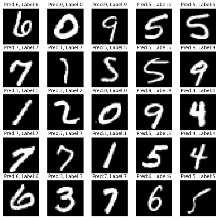
Sample의 idx를 고르는 작업입니다.
sample_indices = np.random.choice(len(mnist_test.targets), n_sample, replace=False)Model에 forward 후 나온 predict값의 argmax(index를 구함)를 출력합니다.
with torch.no_grad():

    y_pred = M.forward(test_x.view(-1, 28, 28).type(torch.float).to(device)/255.)

y_pred = y_pred.argmax(axis=1)
Plt를 사용하여 image를 show합니다.
plt.figure(figsize=(10,10))

for idx in range(n_sample):

    plt.subplot(5, 5, idx+1)

    plt.imshow(test_x[idx], cmap='gray')

    plt.axis('off')

    plt.title("Pred:%d, Label:%d"%(y_pred[idx],test_y[idx]))

plt.show()
'부스트캠프 AI 테크 U stage > 실습' 카테고리의 다른 글
| [16-1] NaiveBayes Classifier Using Konlpy (0) | 2021.02.16 |
|---|---|
| [14-3] Scaled Dot-Product Attention (SDPA) using PyTorch (0) | 2021.02.04 |
| [13-3] Google Image Data 다운로드 (0) | 2021.02.04 |
| [13-2] Colab에서 DataSet 다루기 (강아지 DataSet) (0) | 2021.02.04 |
| [13-1] CNN using PyTorch (0) | 2021.02.04 |


