
| 일 | 월 | 화 | 수 | 목 | 금 | 토 |
|---|---|---|---|---|---|---|
| 1 | 2 | 3 | 4 | 5 | ||
| 6 | 7 | 8 | 9 | 10 | 11 | 12 |
| 13 | 14 | 15 | 16 | 17 | 18 | 19 |
| 20 | 21 | 22 | 23 | 24 | 25 | 26 |
| 27 | 28 | 29 | 30 |
- Numpy data I/O
- type hints
- linalg
- 최대가능도 추정법
- Operation function
- VSCode
- 카테고리분포 MLE
- Python
- subplot
- 부스트캠프 AI테크
- unstack
- 딥러닝
- seaborn
- 가능도
- Comparisons
- groupby
- boolean & fancy index
- python 문법
- Array operations
- 표집분포
- dtype
- Python 특징
- scatter
- BOXPLOT
- namedtuple
- Python 유래
- 정규분포 MLE
- pivot table
- ndarray
- Numpy
- Today
- Total
또르르's 개발 Story
[39-2] Quantization using PyTorch 본문
1️⃣ 설정
모델은 ResNet18, 데이터는 Mnist를 사용합니다.
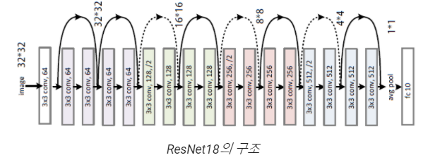
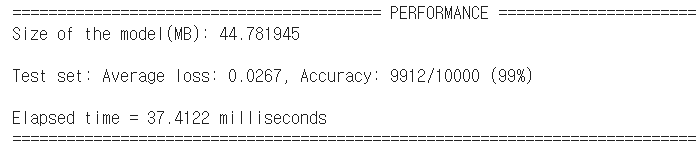
ResNet18에 대한 model의 PERFORMANCE는 다음과 같습니다.
2️⃣ Dynamic Quantization
Dynamic Quantization은 모델의 weight를 quantize 하고, inference 때 레이어의 출력 activation을 더 dynamically quantize (int8) 하게 됩니다.
Dynamic Quantization은 int8 연산 수행(이때 해당 결과는 float32의 형태로 나오는 것을 허용) -> 결과물을 int8로 변환 -> 다시 연산 수행의 과정을 거치게 됩니다.
학습된 모델의 Linear 레이어를 quantize_dynamic로 활용하여 quantizing 해보겠습니다.
(현재 pytorch의 quantize_dynamic 함수는 nn.Linear, nn.LSTM에 대해서만 지원)
# ResNet18의 fully connected layer

self.fc = nn.Linear(512 * block.expansion, num_classes)  # this layer will be quantized later
위 fc layer에 대해 quantization을 수행합니다. ( {nn.Linear} = fc )
quantized_model = torch.quantization.quantize_dynamic(model, {nn.Linear}, dtype=torch.qint8)
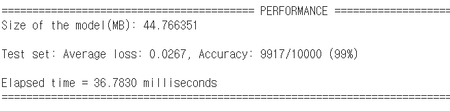
"Original Model"과 "Dynamic quantization을 수행한 Model"을 비교하면 다음과 같습니다.
Latancy (Elapsed time)이 약간 좋아진 것을 알 수 있습니다.
3️⃣ Static Quantization
Static Quantization은 Dynamic Quantization에서 한발 더 나아가, 모든 연산의 결과도 int8의 형태로만 저장하는 quantization 방식입니다. 일반적으로 모델의 학습이 종료된 이후, quantization 효율을 극대화하기 위해 Static Quantization을 사용하게 됩니다.
위에서 학습한 모델을 해당 방식으로 quantizing 해보도록 하겠습니다.
여기서 fuse는 합친다는 의미로 conv와 bn을 합쳐서 사용합니다.
def static_quantize(model, device, test_loader, quantize=False, fbgemm=False):

    model.to(device)

    model.eval()


    modules_to_fuse = [['conv1', 'bn1'],

            ['layer1.0.conv1', 'layer1.0.bn1'],

            ['layer1.0.conv2', 'layer1.0.bn2'],

            ['layer1.1.conv1', 'layer1.1.bn1'],

            ['layer1.1.conv2', 'layer1.1.bn2'],

            ['layer2.0.conv1', 'layer2.0.bn1'],

            ['layer2.0.conv2', 'layer2.0.bn2'],

            ['layer2.0.downsample.0', 'layer2.0.downsample.1'],

            ['layer2.1.conv1', 'layer2.1.bn1'],

            ['layer2.1.conv2', 'layer2.1.bn2'],

            ['layer3.0.conv1', 'layer3.0.bn1'],

            ['layer3.0.conv2', 'layer3.0.bn2'],

            ['layer3.0.downsample.0', 'layer3.0.downsample.1'],

            ['layer3.1.conv1', 'layer3.1.bn1'],

            ['layer3.1.conv2', 'layer3.1.bn2'],

            ['layer4.0.conv1', 'layer4.0.bn1'],

            ['layer4.0.conv2', 'layer4.0.bn2'],

            ['layer4.0.downsample.0', 'layer4.0.downsample.1'],

            ['layer4.1.conv1', 'layer4.1.bn1'],

            ['layer4.1.conv2', 'layer4.1.bn2']]

    model = torch.quantization.fuse_modules(model, modules_to_fuse)

    if fbgemm:

        model.qconfig = torch.quantization.get_default_qconfig('fbgemm')

    else:

        model.qconfig = torch.quantization.default_qconfig

    torch.quantization.prepare(model, inplace=True)

    model.eval()

    with torch.no_grad():

        for data, target in train_loader:

            model(data)

    torch.quantization.convert(model, inplace=True)


    return model
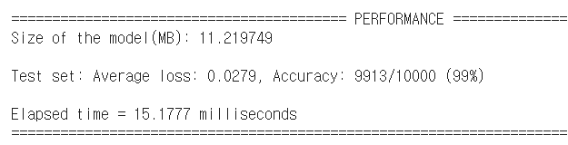
"Original Model"과 "Dynamic quantization을 수행한 Model", "Static quantization을 수행한 Model"을 비교하면 다음과 같습니다.
Latancy (Elapsed time)이 반 이하로 떨어진 것을 볼 수 있고, Model size도 1/4 이하로 떨어진 것을 알 수 있습니다.
그렇다면 Static quantization이 Dynamic quantization보다 좋다고 말할 수 있을까요?
그렇게 볼 수가 없는 것이 이 실험에서는 Dynamic quantization은 fc layer 하나만 quantization을 수행했고, Static quantization은 모든 layer에 대해 수행했기 때문에 비교할 수 없습니다.
4️⃣ qauntized layer histogram
Original 모델과 quantized된 모델의 값이 차이가 나는 부분을 히스토그램으로 표현합니다.
import torch.quantization._numeric_suite as ns

from torch.quantization import (

    default_eval_fn,

    default_qconfig,

    quantize,

)
wt_compare_dict은 weight들을 compare 하기 위해 만든 dictionary입니다.
wt_compare_dict = ns.compare_weights(model.state_dict(), quantized_model.state_dict())


>>> print(wt_compare_dict.keys())

dict_keys(['conv1.weight', 'layer1.0.conv1.weight', 'layer1.0.conv2.weight', 'layer1.1.conv1.weight', 'layer1.1.conv2.weight', 'layer2.0.conv1.weight', 'layer2.0.conv2.weight', 'layer2.0.downsample.0.weight', 'layer2.1.conv1.weight', 'layer2.1.conv2.weight', 'layer3.0.conv1.weight', 'layer3.0.conv2.weight', 'layer3.0.downsample.0.weight', 'layer3.1.conv1.weight', 'layer3.1.conv2.weight', 'layer4.0.conv1.weight', 'layer4.0.conv2.weight', 'layer4.0.downsample.0.weight', 'layer4.1.conv1.weight', 'layer4.1.conv2.weight', 'fc._packed_params._packed_params'])


>>> print(wt_compare_dict['conv1.weight'].keys())

dict_keys(['float', 'quantized'])


>>> print(wt_compare_dict['conv1.weight']['float'].shape)

torch.Size([64, 1, 7, 7])


>>> print(wt_compare_dict['conv1.weight']['quantized'].shape)

torch.Size([64, 1, 7, 7])
conv1의 weight에 대한 quantize된 값과 float 된 값을 histogram으로 그립니다.
비슷해 보이지만, x축과 y축의 범위가 다르다는 것을 알 수 있습니다.
histogram의 x축 scale을 보면 quantized의 x축이 더 늘어난 것을 알 수 있습니다.
또한, quantize는 비슷한 값끼리 하나로 모아서 묶기 때문에 y축의 값들도 float보다 늘어난 것을 볼 수 있습니다.
# quantized

plt.figure(figsize=(30, 5))

q = wt_compare_dict['conv1.weight']['quantized'].flatten().dequantize()

plt.hist(q, bins = 100)

plt.title("Quantized model weights of conv1")

plt.show()


# float

plt.figure(figsize=(30, 5))

f = wt_compare_dict['conv1.weight']['float'].flatten()

plt.hist(f, bins = 100)

plt.title("Floating point model weights of conv1")

plt.show()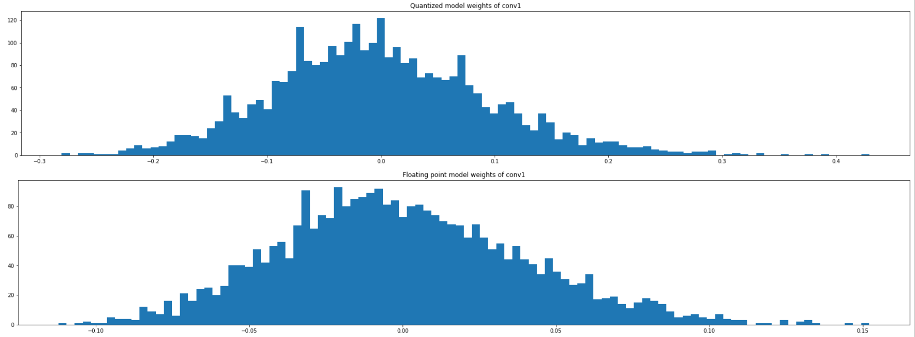
quantized 된 histogram을 파란색, float된 histogram을 주황색으로 표현하면 다음과 같습니다.
plt.figure(figsize=(25, 7))

q = wt_compare_dict['conv1.weight']['quantized'].flatten().dequantize()

plt.hist(q, bins = 100)

#plt.title("Quantized model weights of conv1")


f = wt_compare_dict['conv1.weight']['float'].flatten()

plt.hist(f, bins = 100)

plt.title("Comparing the weights of two conv1 layers")


plt.show()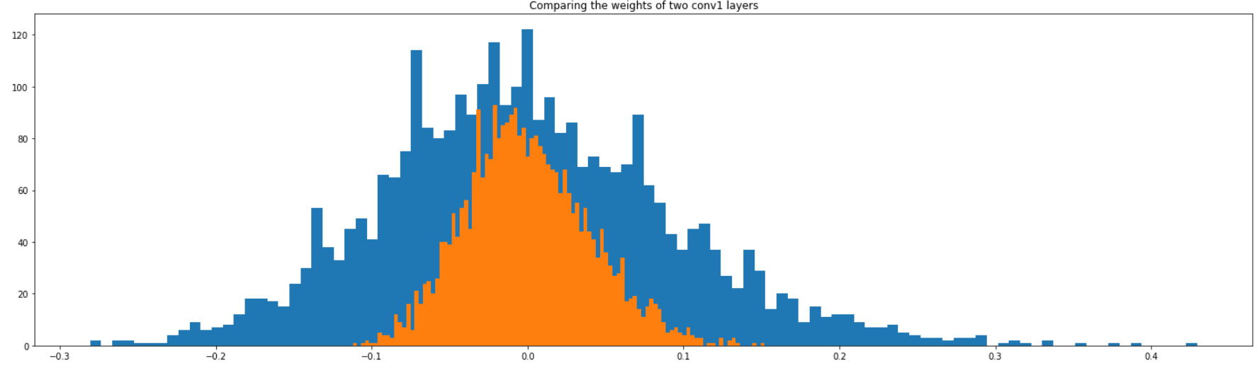
'부스트캠프 AI 테크 U stage > 실습' 카테고리의 다른 글
| [39-3] Teacher-Student Network using PyTorch (0) | 2021.03.19 |
|---|---|
| [38-3] Pruning using PyTorch (0) | 2021.03.18 |
| [38-2] Python 병렬 Processing (0) | 2021.03.17 |
| [37-2] PyTorch profiler (0) | 2021.03.17 |
| [36-1] Model Conversion (0) | 2021.03.16 |


