
| 일 | 월 | 화 | 수 | 목 | 금 | 토 |
|---|---|---|---|---|---|---|
| 1 | 2 | 3 | 4 | 5 | ||
| 6 | 7 | 8 | 9 | 10 | 11 | 12 |
| 13 | 14 | 15 | 16 | 17 | 18 | 19 |
| 20 | 21 | 22 | 23 | 24 | 25 | 26 |
| 27 | 28 | 29 | 30 |
- Python 유래
- type hints
- 표집분포
- dtype
- 딥러닝
- 정규분포 MLE
- 부스트캠프 AI테크
- Python 특징
- groupby
- scatter
- BOXPLOT
- ndarray
- VSCode
- 최대가능도 추정법
- Numpy
- linalg
- unstack
- boolean & fancy index
- 카테고리분포 MLE
- Array operations
- pivot table
- Python
- namedtuple
- Operation function
- python 문법
- Numpy data I/O
- 가능도
- subplot
- seaborn
- Comparisons
- Today
- Total
또르르's 개발 Story
[08] Python pandas (1) 본문
Pandas는 panel data의 줄임말로 파이썬의 데이터 처리의 사실상 표준인 라이브러리입니다.
Python의 pandas는 통계 프로그램인 R하고 비슷하다는 소리를 많이 듣는데요.
pandas의 객체 생성과 함수들을 정리해보았습니다.
1️⃣ Pandas 개요
1) Pandas 특징
- 구조화된 데이터 처리를 지원하는 Python 라이브러리
- Numpy와 통합하여 ndarray를 사용할 수 있고, 강력한 "스프레드시트" 처리 기능 제공
- 인덱싱, 연산용 함수, 전처리 함수 등 제공
- 데이터 처리 및 통계 분석을 위해 사용
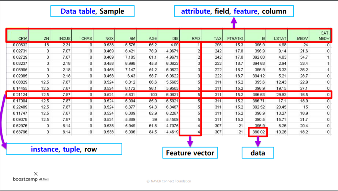
2) 스프레드시트 구성요소
- Data table, Sample : Data Frame 표 전체를 말함
- attribute, field, feature, column : 열(column)의 이름을 말함
- instance, tuple, row : 행(row)으로써 하나의 줄
- data : 숫자나 문자로 표현된 하나의 단위
아래 그림과 같이 엑셀 형태의 Data table을 Tabular라고 합니다.
3) Pandas 데이터 로딩
CSV 타입의 데이터를 로드합니다. (sep는 sperate 형식 지정, header는 Column이름을 설정합니다.)
data_url = 'https://archive.ics.uci.edu/ml/machine-learning-databases/housing/housing.data' #Data URL
# data_url = "./housing.data"
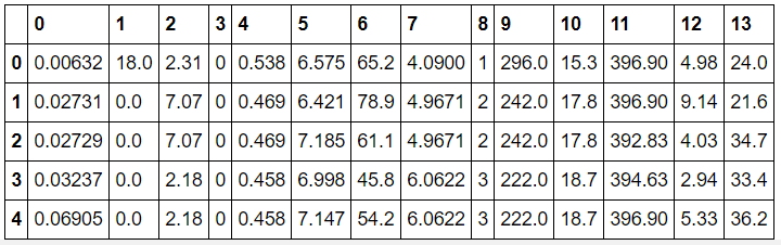
>>> df_data = pd.read_csv(data_url, sep="\s+", header=None) # sep = 나누는 sentence (single space 연속)head()를 사용하면 data frame을 출력합니다.
>>> df_data.head(5) # 처음 다섯줄 출력
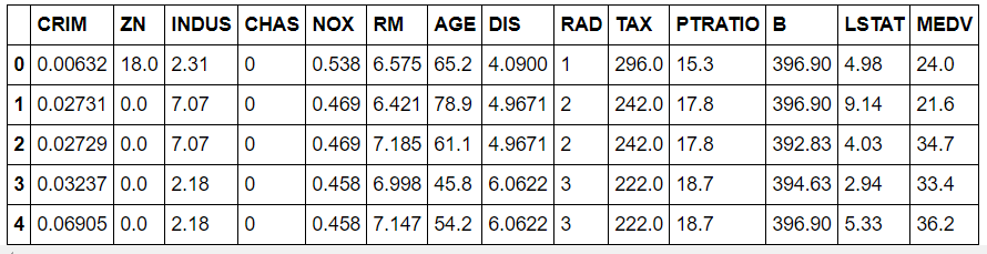
또한 columns=[ ]를 사용하면 Column의 이름을 지정할 수 있습니다.
df_data.columns = [
    "CRIM",
    "ZN",
    "INDUS",
    "CHAS",
    "NOX",
    "RM",
    "AGE",
    "DIS",
    "RAD",
    "TAX",
    "PTRATIO",
    "B",
    "LSTAT",
    "MEDV",
]
2️⃣ Pandas object
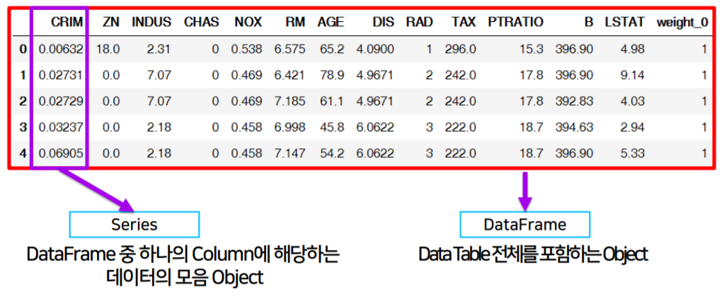
1) Pandas 구성요소
- Series : Data frame의 하나의 Column에 해당하는 데이터 모음 object
- Data frame : Data table 전체를 포함하는 object
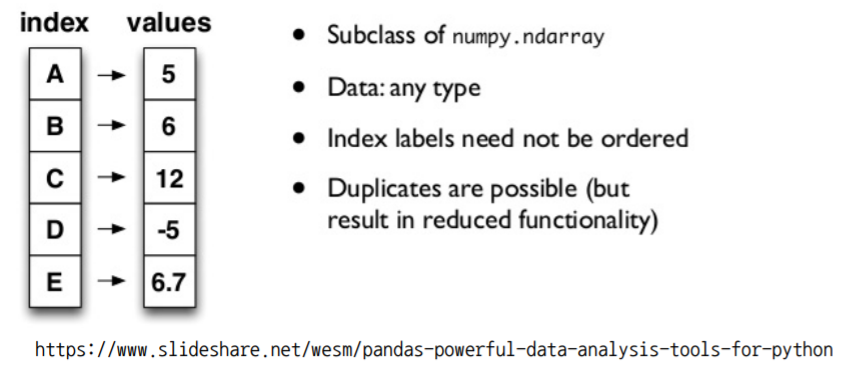
2) Series
Series는 Data frame에서 Column vector를 표현하는 object입니다.
index가 추가된 numpy.ndarray라고 생각하시면 편합니다.
- 생성
list를 사용해서 Series를 만들 수 있습니다.
이 때 Series의 index를 명시하지 않으면 자동 생성됩니다.
>>> list_data = [1, 2, 3, 4, 5]

>>> example_obj = Series(data=list_data)

>>> example_obj

0    1
1    2
2    3
3    4
4    5
dtype: int64
dict을 가지고 Series를 생성할 수 있습니다.
>>> dict_data = {"a": 1, "b": 2, "c": 3, "d": 4, "e": 5}

>>> example_obj = Series(dict_data, dtype=np.float32, name="example_data")

>>> example_obj

a    3.0
b    2.0
c    3.0
d    4.0
e    5.0
Name: example_data, dtype: float32
- Index
Series에 index 이름을 설정할 수 있습니다.
>>> list_data = [1, 2, 3, 4, 5]

>>> list_name = ["a", "b", "c", "d", "e"]

>>> example_obj = Series(data=list_data, index=list_name)

>>> example_obj

a    1
b    2
c    3
d    4
e    5
dtype: int64
Series에서는 index를 기준으로 칸이 생성이 됩니다.
만약 index는 있지만 data가 없는 칸은 NaN으로 출력됩니다.
>>> dict_data = {"a": 1, "b": 2, "c": 3, "d": 4, "e": 5}

>>> indexes = ["a", "b", "c", "d", "e", "f", "g", "h"]

>>> example_obj = Series(dict_data, index=indexes)

>>> example_obj

a    1.0
b    2.0
c    3.0
d    4.0
e    5.0
f    NaN
g    NaN
h    NaN
dtype: float32
- 메서드
- values : 값 리스트만 출력
>>> example_obj.index

array([1., 2., 3., 4., 5. ], dtype=float32)
- index : index 리스트만 출력
>>> example_obj.values

Index(['a', 'b', 'c', 'd', 'e'], dtype='object')
- astype : Series의 dtype을 변경
>>> example_obj = example_obj.astype(float)

>>> example_obj["a"] = 3.2

>>> example_obj

a    3.2
b    2.0
c    3.0
d    4.0
e    5.0
dtype: float64
- to_dict : Series가 dict_type으로 변경
>>> example_obj.to_dict()

{'a': 3.2, 'b': 2.0, 'c': 3.0, 'd': 4.0, 'e': 5.0}
또한, Boolean index와 Fancy index 사용이 가능합니다.
>>> cond = example_obj > 2

>>> example_obj[cond]

a    3.2
c    3.0
d    4.0
e    5.0
dtype: float64
>>> example_obj[example_obj > 2]
a 3.2
c 3.0
d 4.0
e 5.0
dtype: float64
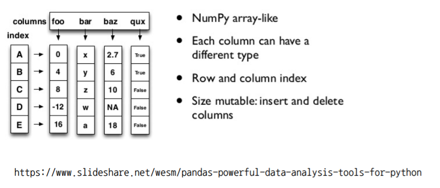
3) Data frame
Data frame은 Data table 전체를 의미하며 Series의 집합입니다.
따라서 Series마다 다른 dtype을 가질 수 있습니다.
- 생성
dict_type을 사용해서 data frame을 만들 수 있습니다. (하지만 대부분 data를 load해서 사용합니다.)
raw_data = {
    "first_name": ["Jason", "Molly", "Tina", "Jake", "Amy"],
    "last_name": ["Miller", "Jacobson", "Ali", "Milner", "Cooze"],
    "age": [42, 52, 36, 24, 73],
    "city": ["San Francisco", "Baltimore", "Miami", "Douglas", "Boston"],
}

>>> df = pd.DataFrame(raw_data, columns=["first_name", "last_name", "age", "city"])

>>> df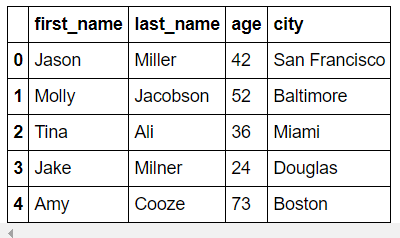
- Index
Data frame에서 Column을 선택할 수 있습니다.
>>> DataFrame(raw_data, columns=["age", "city"])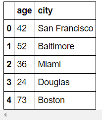
Data frame에서 Columns를 추가할 수 있습니다.
(실제로 추가된 것은 아니며, 값이 없으므로 NaN으로 표시됩니다.)
>>> DataFrame(raw_data, columns=["first_name", "last_name", "age", "city", "debt"])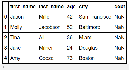
또한. Column이름을 사용해서 Column을 선택해 출력할 수 있습니다.
>>> df.first_name

0    Jason
1    Molly
2     Tina
3     Jake
4      Amy
Name: first_name, dtype: object
>>> df["first_name"]
0 Jason
1 Molly
2 Tina
3 Jake
4 Amy
Name: first_name, dtype: object
- 메서드
- loc : index location의 약자로 index이름으로 값을 찾음
두 번째 parameter는 원하는 column 출력을 명시할 수 있으며, list형태입니다.
>>> df.loc[:, ["last_name"]]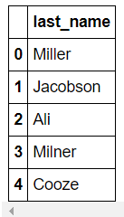
- iloc : index position의 약자로 index의 number로 값을 찾음
>>> df["age"].iloc[1:]


1    52
2    36
3    24
4    73
Name: age, dtype: int64
✅ loc과 iloc의 차이는 data frame에서 index의 이름을 생성할 수 있기 때문에 일어납니다.
loc은 index의 이름을 따라가며, iloc은 index의 순서를 따라갑니다.
예를 들어, s라는 Series가 존재할 때
s = pd.Series(np.nan, index=[49, 48, 47, 46, 45, 1, 2, 3, 4, 5])loc은 [:3]을 하면 index의 이름이 '3'인 것(전에 있는 것)을 불러옵니다.
>>> s.loc[:3]

49   NaN
48   NaN
47   NaN
46   NaN
45   NaN
1    NaN
2    NaN
3    NaN
dtype: float64
iloc은 [:3]을 하게되면 3번째 있는 값(전에 있는 것)을 불러옵니다.
>>> s.iloc[:3]

49   NaN
48   NaN
47   NaN
dtype: float64
- T : transpose
>>> df.head(3).T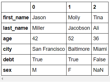
- to_csv : csv로 변환
>>> df.to_csv()

',first_name,last_name,age,city,debt,sex\r\n0,Jason,Miller,42,San Francisco,True,M\r\n1,Molly,Jacobson,52,Baltimore,True,F\r\n2,Tina,Ali,36,Miami,False,\r\n3,Jake,Milner,24,Douglas,False,F\r\n4,Amy,Cooze,73,Boston,True,\r\n'
- reset_index : 초기화된 index가 들어감
>>> df.reset_index()>>> df.reset_index(drop=True) # 기존 index를 삭제하고 초기화된 index가 들어감
또한, Boolean index와 Fancy index 사용이 가능합니다.
>>> df.debt = df.age > 40		# debt column에 True, False로 삽입

>>> df
3️⃣ Selection & drop
데이터 처리에서 가장 중요한 Selection과 drop에 대해서 알아보겠습니다.
1) Selection
하나 이상의 Column을 선택할 때는 list를 사용합니다.
>>> df[["first_name", "age","city"]].head(3)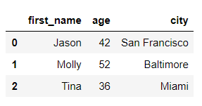
Column의 이름없이 출력할 때는 index number가 같이 출력됩니다.
>>> df[:3]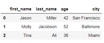
Column 이름과 함께 출력할 때는 해당 column의 row index가 출력됩니다.
>>> df["first_name"][:3]

0    Jason
1    Molly
2     Tina
Name: first_name, dtype: object
✅ df["account"]와 df[["account"]] 차이
df["account"] : 문자로 출력
df[["account"]] : data frame 형태로 출력
loc과 iloc을 사용해서 data frame을 선택할 수 있습니다.
(loc은 column이름을 명시해야되지만 iloc은 명시할 필요가 없습니다.)
>>> df.loc[[211829, 320563], ["name", "street"]]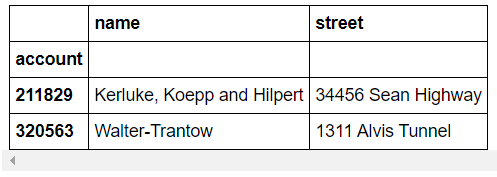
>>> df.iloc[:10, :3]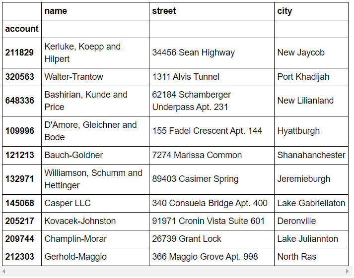
2) drop
drop은 index number을 사용해서 drop 합니다.
>>> df.drop(1) # 1번 행 삭제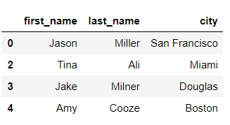
list를 사용해서 여러 행을 삭제합니다.
>>> df.drop([0,1,2,3]) # 1,2,3,4번 행 삭제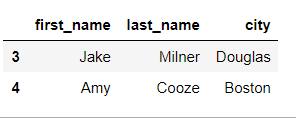
axis 축을 지정해서 Column을 삭제할 수 있습니다.
>>> df.drop("city", axis=1)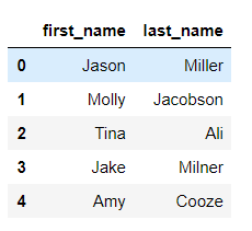
✅ Drop을 사용하면 실제 Data frame에서 값이 삭제가 되나요?
삭제되지 않습니다. drop을 실행하면 출력만 그렇게 보입니다.
만약, 실제 Data frame에서 삭제하고 싶다면 parameter에 inplace=True를 추가하세요.
>>> df.drop([0,1,2], inplace=True)

>>> df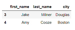
4️⃣ Data frame operation
데이터 프레임은 기본적인 사칙연산('+' = add, '-' = sub, '*' = mul, '/' = div)을 지원합니다.
s1 = Series(range(1, 6), index=list("abced"))s2 = Series(range(5, 11), index=list("bcedef"))>>> s1 + s2
a NaN
b 7.0
c 9.0
d 13.0
e 11.0
e 13.0
f NaN
dtype: float64>>> s1.add(s2)
a NaN
b 7.0
c 9.0
d 13.0
e 11.0
e 13.0
f NaN
dtype: float64
두 data frame의 모양이 다른 경우 data가 없는 곳에는 NaN으로 표시됩니다.
df1 = DataFrame(np.arange(9).reshape(3, 3), columns=list("abc"))

>>> df1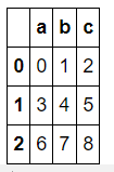
df2 = DataFrame(np.arange(16).reshape(4, 4), columns=list("abcd"))

>>> df2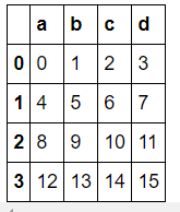
>>> df1 + df2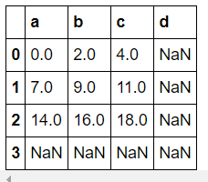
위와 같은 경우 add method의 fill_value=0를 사용하면 해결이 가능합니다.
(데이터가 NaN인 경우 0으로 설정)
>>> df1.add(df2, fill_value=0)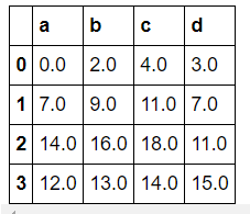
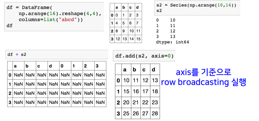
또한, axis를 사용해서 행(axis=0)에 더하는 것이 가능합니다.
이때 s2의 크기는 df와 같지 않으므로 broadcasting(shape을 맞추기 위해 값을 복사)을 수행합니다.
(s2를 복사해서 df와 같은 모양으로 만든 다음 df+s2(axis=0)를 실행)
5️⃣ Map, Apply
1) map : 함수를 받아 계산된 object 반환
def f(x):
    return x + 5


>>> s1.map(f)

0     5
1     6
2     7
3     8
4     9
5    10
6    11
7    12
8    13
9    14
dtype: int64
dict_type을 map으로 넣었을 때 dict의 key값을 value의 값으로 변환해줍니다.
z = {1: "A", 2: "B", 3: "C"}

>>> s1.map(z)

0    NaN
1      A
2      B
3      C
4    NaN
5    NaN
6    NaN
7    NaN
8    NaN
9    NaN
dtype: object
map 대신 replace 함수를 사용하기도 합니다.
>>> df.sex.replace({"male": 0, "female": 1})

0       0
1       1
2       1
3       1
4       1
       ..
1374    0
1375    1
1376    1
1377    0
1378    0
Name: sex, Length: 1379, dtype: int64
>>> df.sex.replace(["male", "female"], [0, 1], inplace=True)
# sex라는 column에서 male는 0으로 female는 1로 변환하고 실제 data를 변경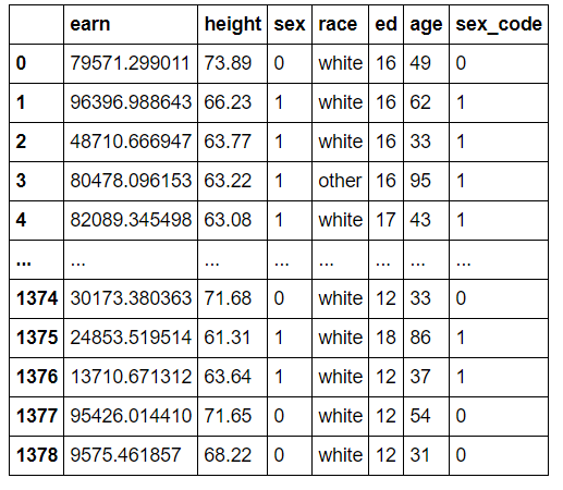
2) apply : 함수를 입력받아 각 Column별로 결과값을 반환
>>> f = lambda x: np.mean(x)	# mean을 구하는 함수

>>> df_info.apply(f)		# 각 column별로 mean을 구해 반환

earn      32446.292622
height       66.592640
age          45.328499
dtype: float64
내장함수 sum, mean, std도 사용이 가능합니다.
>>> df_info.apply(np.mean)

earn      32446.292622
height       66.592640
age          45.328499
dtype: float64
Series 형태로 반환하면 원하는 형태의 값으로 출력이 가능합니다.
def f(x):
    return Series(
        [x.min(), x.max(), x.mean(), sum(x.isnull())],
        index=["min", "max", "mean", "null"],
    )


>>> df_info.apply(f)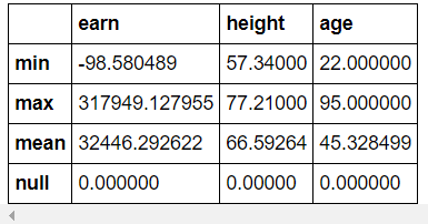
6️⃣ Pandas built-in functions
1) descirbe : Numeric type 데이터의 요약 정보를 보여줌
>>> df.describe()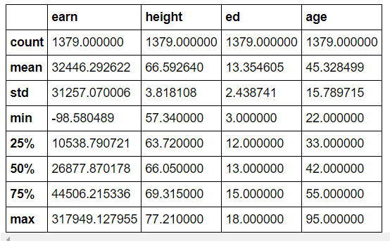
2) unique : series data의 유일한 값을 list로 반환
>>> df.race.unique()

array(['white', 'other', 'hispanic', 'black'], dtype=object)
3) sum : axis 설정을 통해 row와 column 합 지원
>>> df.sum(axis=1)	# row를 기준으로 출력

0       79710.189011
1       96541.218643
2       48823.436947
3       80652.316153
4       82212.425498
            ...
1374    30290.060363
1375    25018.829514
1376    13823.311312
1377    95563.664410
1378     9686.681857
Length: 1379, dtype: float64
4) isnull() : column 또는 row 값의 NaN 값의 index 반환
>>> df.isnull().sum() / len(df)  # df 전체에서 null값의 비중을 알 수 있음

earn      0.0
height    0.0
sex       0.0
race      0.0
ed        0.0
age       0.0
dtype: float64
5) sort_values : column값 기준으로 데이터 sorting
>>> df.sort_values(["age", "earn"], ascending=True)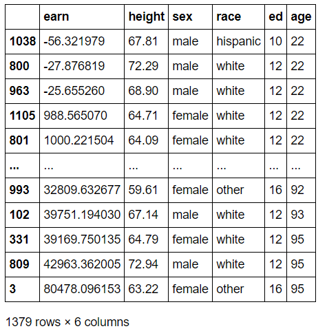
6) Corr, cov, corrwith : 상관계수, 공분산
>>> df.age.corr(df.earn)

0.07400349177836055
>>> df.age[(df.age < 45) & (df.age > 15)].corr(df.earn)
0.31411788725189044>>> df.age.cov(df.earn)
36523.6992104089
[09] Python pandas (2)
[08] Python pandas (1) Pandas는 panel data의 줄임말로 파이썬의 데이터 처리의 사실상 표준인 라이브러리입니다. Python의 pandas는 통계 프로그램인 R하고 비슷하다는 소리를 많이 듣는데요. pandas의 객체
dororo21.tistory.com
Python pandas(2)에서 이어집니다....
'부스트캠프 AI 테크 U stage > 이론' 카테고리의 다른 글
| [09] Python pandas (2) (0) | 2021.01.28 |
|---|---|
| [08-1] 신경망(neural network) (0) | 2021.01.27 |
| [07] 경사하강법 (0) | 2021.01.26 |
| [06-1] 벡터와 행렬 with Python Numpy (0) | 2021.01.25 |
| [06] Python numpy (1) | 2021.01.25 |


